
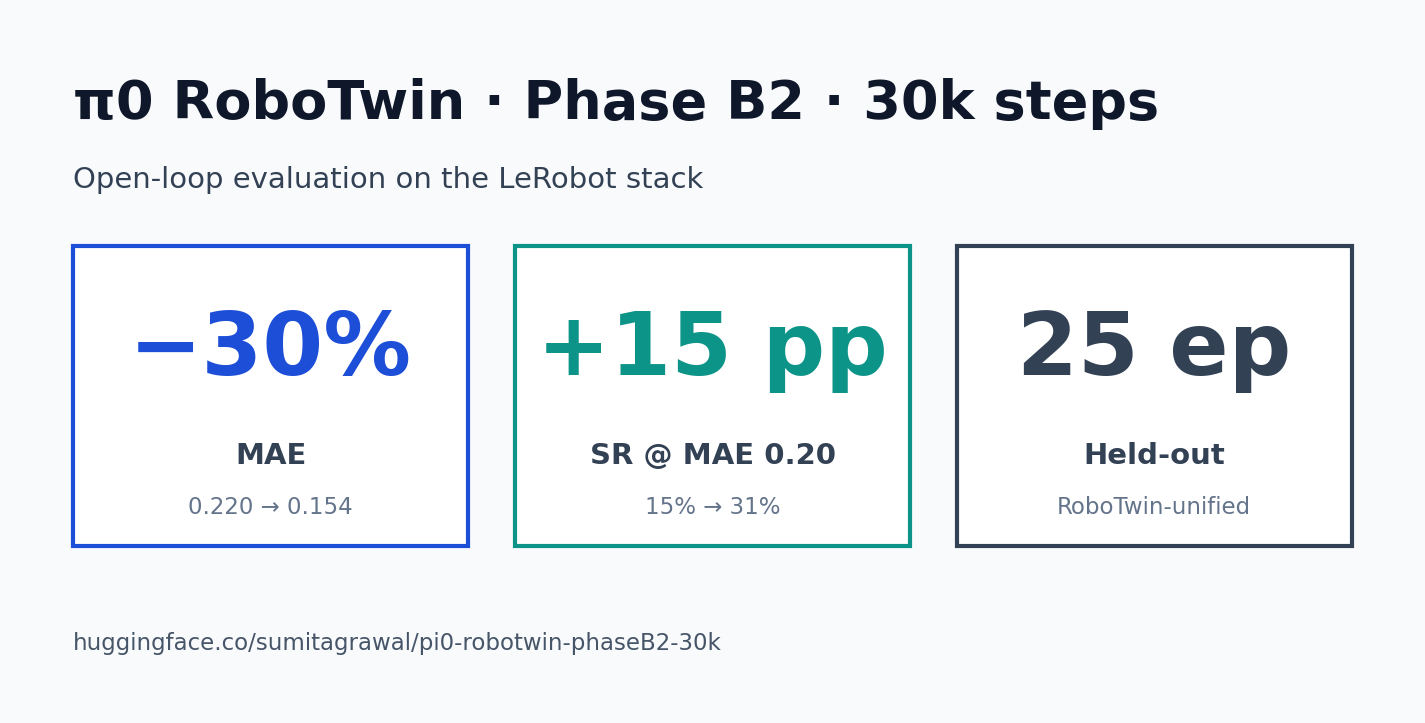
TL;DR — Key Takeaways
- Phase B2 ≠ Phase B. Same
lerobot/pi0_basestart, same RoboTwin-unified data, same 30k steps — different recipe. Phase B2 cut aggregate open-loop MAE by 30% (0.220 → 0.154) and roughly doubled SR @ MAE 0.20 (15% → 31%) on held-out episodes. - Eval, not vibes. Both runs use the LeRobot open-loop harness: re-create the policy with
PI0Policy.from_pretrained(...), replay held-out RoboTwin trajectories, score MSE/MAE per joint plus step success rates at thresholds. - Right arm got the most help. Per-joint MAE drops the most on joints 7–13 (right arm + grip), where Phase B was clearly weaker.
- Action plots show what the metrics hide. A pred-vs-gt overlay for episode
22042shows the policy tracking gross trajectories well, with a mid-episode discontinuity that pulls average MAE up. - Weights are public. The Phase B2 30k checkpoint lives at
sumitagrawal/pi0-robotwin-phaseB2-30k—PI0Policy.from_pretrained(...)and you’re running.
Why Open-Loop Eval (and Why It’s Honest)
π0 is a vision-language-action policy: cameras + state + a task string in, action chunks out. The cleanest way to measure “did this fine-tune learn something?” without a sim wrapper is open-loop replay:
- Take a held-out episode from the same dataset family.
- At each step, give the policy the real observation.
- Have it predict the next action chunk.
- Score the chunk against the recorded ground-truth actions.
It doesn’t close the loop on physics — that needs a sim or robot. But it isolates the policy’s behavior from compounding sim error and gives you per-step, per-joint numbers you can actually compare across runs.
The two runs in this post:
| Run | Checkpoint | Episodes | Aggregate MAE | Aggregate MSE | Runtime |
|---|---|---|---|---|---|
| Phase B | pi0-phaseB-20260503-205352 / 030000 |
5 | 0.2202 | 0.1960 | 9 min |
| Phase B2 | pi0-phaseB2-20260505-151435 / 030000 |
25 | 0.1543 | 0.1283 | 42 min |
Same base model. Same step count. Phase B was the smaller pilot; Phase B2 used the refined recipe and a wider eval slice.
The Headline Numbers
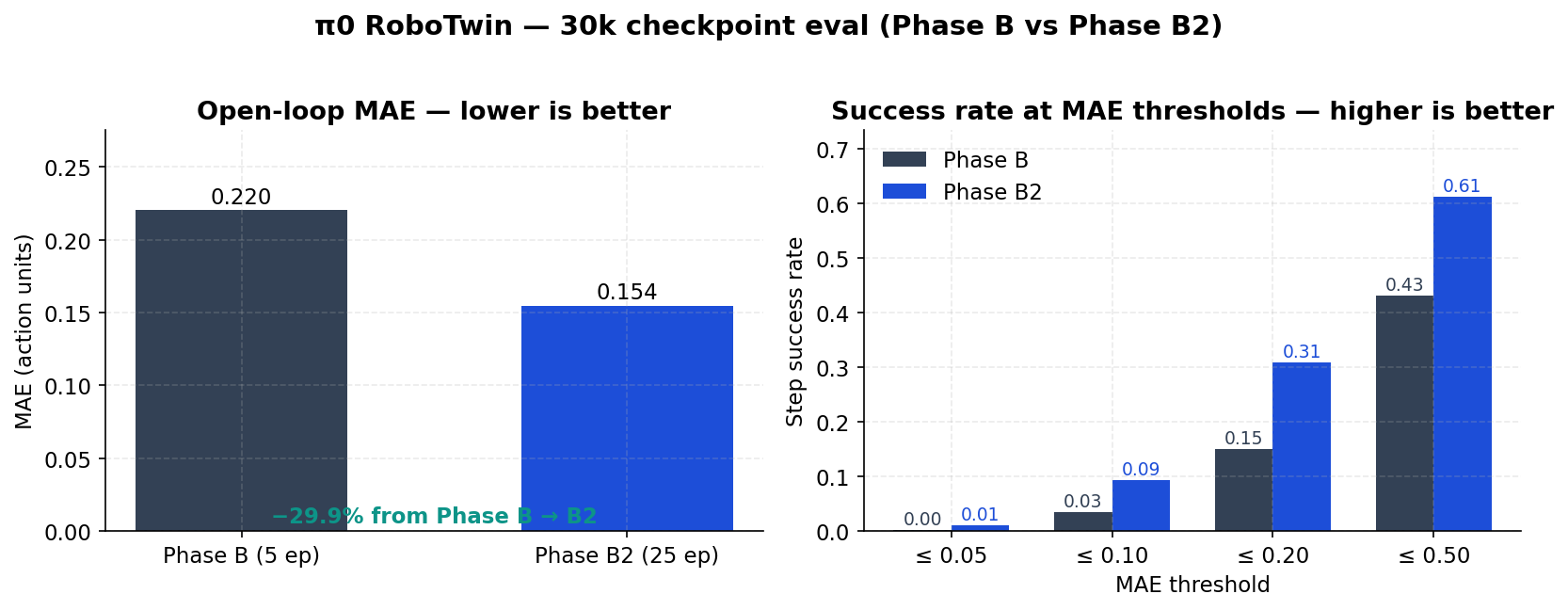
Two complementary views: MAE (lower is better) and success rate at MAE thresholds (higher is better). The success rate at threshold t is the fraction of steps where the per-step MAE is ≤ t — a forgiving but useful proxy for “did the policy at least stay in the neighborhood?”.
| Metric | Phase B | Phase B2 | Δ |
|---|---|---|---|
| Aggregate MAE | 0.2202 | 0.1543 | −30.0 % |
| Aggregate MSE | 0.1960 | 0.1283 | −34.5 % |
| SR @ MAE 0.05 | 0.1 % | 1.0 % | +0.9 pp |
| SR @ MAE 0.10 | 3.4 % | 9.4 % | +6.0 pp |
| SR @ MAE 0.20 | 15.1 % | 30.9 % | +15.8 pp |
| SR @ MAE 0.50 | 43.2 % | 61.1 % | +18.0 pp |
The 0.20 threshold is the most operational: it’s the band where the policy is still “close enough” for replay in a sim controller, before chunk re-planning kicks in.
Where the Improvement Lives: Per-Joint MAE
ALOHA-style 14-DoF actions: j0–j6 are the left arm + gripper, j7–j13 are the right arm + gripper. The two runs’ per-joint MAE side by side:
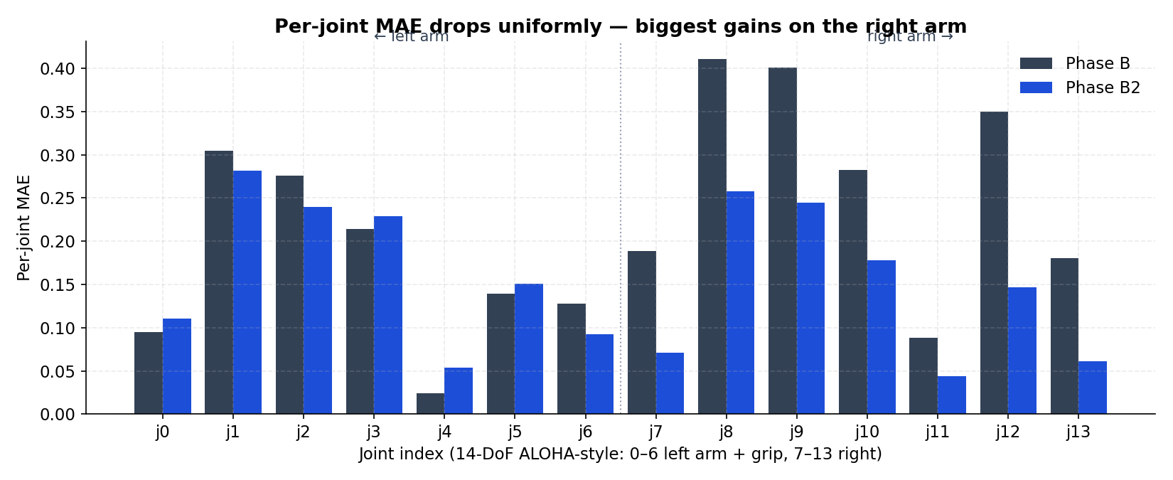
- Phase B already did fine on
j4(a near-static gripper-axis joint). - The biggest absolute drops show up on
j8,j9,j12— right-arm joints that involve wider, multi-second motions. Phase B was wobbly there; B2 tightened the tracking. - Left arm (
j0–j6) improved more modestly; it was already in a good place.
This is exactly what you want a refinement run to look like: focused improvement on the weakest joints, no regressions elsewhere.
How Consistent Is It? Per-Episode MAE on Phase B2
Five episodes is a story. 25 is a starter distribution.
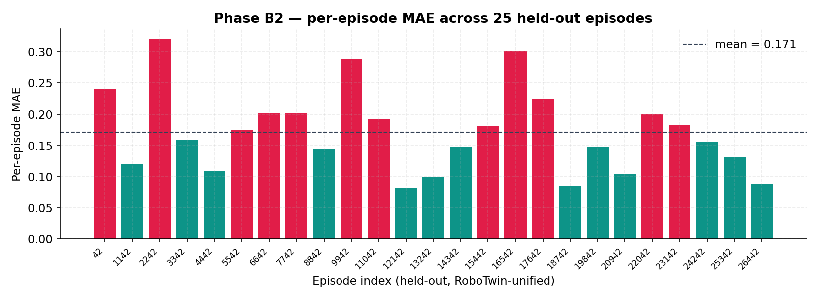
Bars below the dashed mean line are coloured teal (better than average), above it rose. Most episodes cluster around 0.10–0.20 MAE, with a few outliers near 0.30 (longer or harder-to-track tasks).
That long tail is informative — it tells you which episode types to target next (more data, weighted sampling, or a curriculum bump on those task IDs).
What Open-Loop Looks Like (Episode 22042)
This is the per-step prediction overlay for one of the harder episodes:
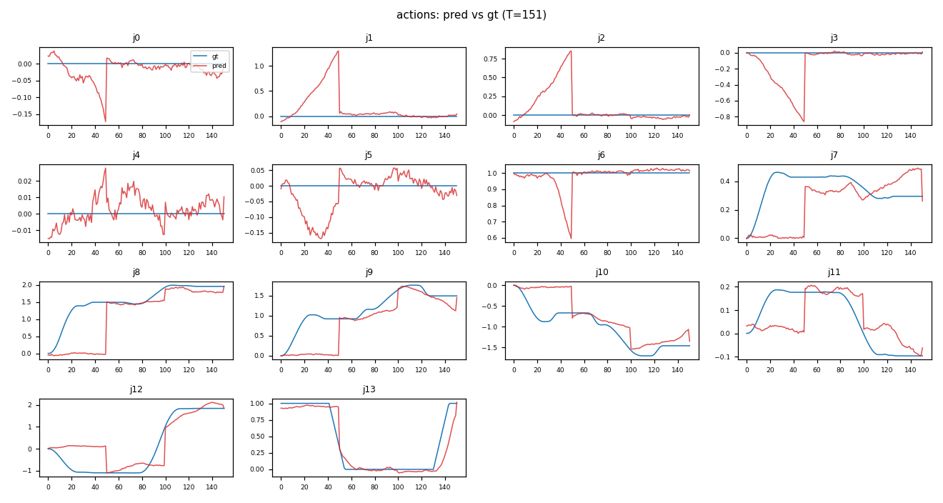
A few things stand out:
- Most joints (
j8–j13, much ofj0) show the predicted (red) curve hugging the ground-truth (blue) shape over the full 151-step window. - Around step ~50 several joints have a sharp discontinuity — the predicted chunk transitions don’t line up perfectly with a ground-truth contact event. That single window is responsible for a meaningful chunk of episode-level MAE.
- The static joints (
j4,j6) sit near zero with low-amplitude jitter — expected.
That mid-episode jump is a familiar failure mode for open-loop eval: chunked action policies are planning-ahead models, and a 1-step shift in when a contact is predicted can produce a tall, brief MAE spike that dominates the episode score.
A short rollout from the same episode (10 fps, 720p):
The Pipeline
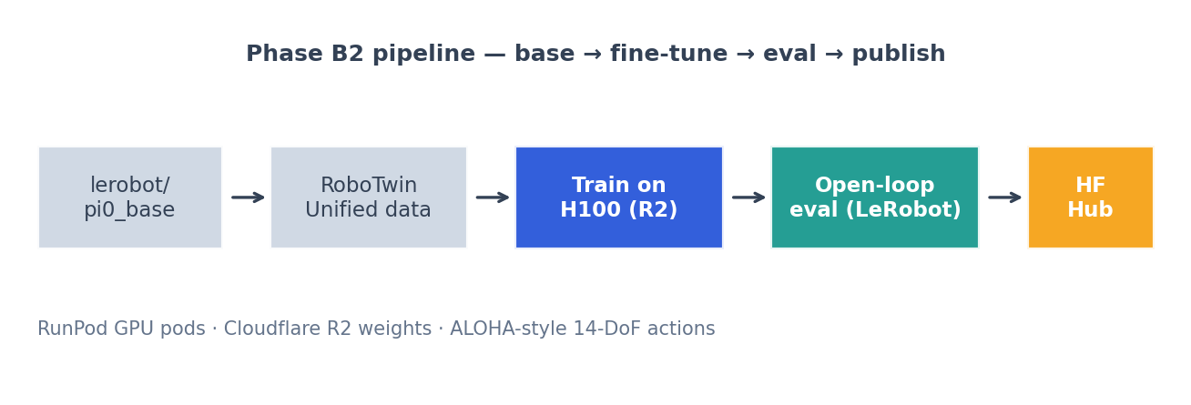
- Base.
lerobot/pi0_base. - Data. RoboTwin-unified — the LeRobot-format aggregated RoboTwin set (
lerobot/robotwin_unified). - Train. RunPod H100 pod, weights/checkpoints staged on Cloudflare R2 so spot interruptions don’t cost progress. 30k steps of standard π0 fine-tuning.
- Eval. A small open-loop harness using
LeRobotDataset+PI0Policy.from_pretrained(...)+make_pre_post_processors(...), run on the030000checkpoint. - Publish. Stage
pretrained_model/(weights + tokenizer/preprocessor shards) + a model card →huggingface_hub.upload_folder→ public Hub repo.
The training compute and data prep are the patient parts. The eval-and-publish loop is fast — minutes once you have a checkpoint you trust.
Using the Model
from lerobot.policies.pi0.modeling_pi0 import PI0Policy

policy = PI0Policy.from_pretrained("sumitagrawal/pi0-robotwin-phaseB2-30k")
policy.eval()
# Build observation batch from your robot (or LeRobotDataset row):
#   observation.images.*  — multi-camera tensors
#   observation.state     — robot state vector
#   task                  — language instruction string
# Use make_pre_post_processors(policy_cfg=policy.config, pretrained_path=<repo>)
# to wire input/output normalization correctly.
For an end-to-end working example (load → build batch from a dataset row → first action chunk), the same training repo ships an inference_pi0_from_hub.py you can adapt.
What I’d Do Next
- Sim-in-the-loop. Open-loop is a screening tool; closed-loop in a RoboTwin sim is where these MAE numbers translate to real task success.
- Targeted data on weak episodes. The 25-episode distribution surfaces a few stubborn outliers — those are the next batch to over-sample (or to inspect for label issues).
- Chunk-aware loss tweaks. The mid-episode discontinuity in episode
22042is classic chunked-policy behavior; a small loss term on chunk-boundary smoothness might help. - Bigger eval, public artifacts. 50–100 episodes is the next bar, with the metrics + plots committed alongside the model card so anyone can reproduce.
Honest Caveats
- This is open-loop. Real task success requires sim or hardware.
- The two runs differ in eval breadth (5 ep vs 25 ep). The B2 distribution is the truer picture; B is a pilot baseline.
- The dataset and base model carry their own licenses/limits — see
lerobot/pi0_baseandlerobot/robotwin_unifiedon the Hub. - “Same 30k steps” doesn’t mean “same total compute” — recipe differences (LR schedule, batch composition, augmentation) account for the lift.
Links
- Model:
sumitagrawal/pi0-robotwin-phaseB2-30kon Hugging Face - Base model:
lerobot/pi0_base - LeRobot: github.com/huggingface/lerobot
- RoboTwin-unified:
lerobot/robotwin_unified
If you spin this up on your own robot or sim and the numbers look different — please share. Open-loop is a starting line, not a finish line.